Time for a bit of a change of pace. Solver is by far the coolest thing I have learned on Excel in recent memory. I still don’t really understand how it works, but the instructions here will allow you to identify certain numbers in a list of numbers that add to a desired result.
Say you have a big list of data (e.g. bank transactions) that looks something like this:

In this example, we have 30 lines of data. A certain combination of these results in 37,161. We want to know which ones will do that.
Switches
This Solver method works on ‘switching’ the appropriate zeros to ones. This will make more sense later but for now, just throw some zeros against each line of data.
SumProduct
If you aren’t familiar with SumProduct don’t worry about it too much. I’ve never used it before this. You can learn more about the function on your own, but for cell D3 the formula is =SUMPRODUCT(A2:A31,B2:B31).
Goal
Simply the number you are aiming for. Manual input.
Variance
Just the difference between the SumProduct cell and the Goal cell.
SOLVER
First thing you’ll need to do is enable the Solver add-in (File > Options > Add-Ins > Pick “Excel Add-ins” from the drop-down menu > Go > Select the “Solver Add-in” checkbox > OK) then open it up in the Data tab.

Without over-explaining things (because I don’t understand how this works and think it’s still mostly magic) this is what your dialogue box should look like:
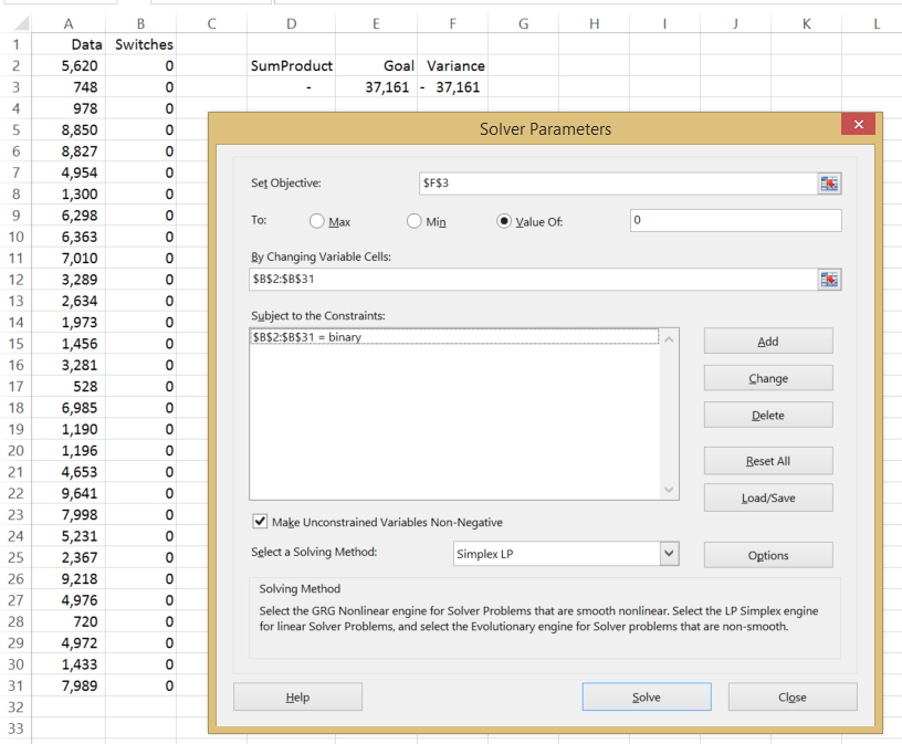
Then hit Solve. The magic Solver pixies will flick the switches of the numbers that add to your specified goal.
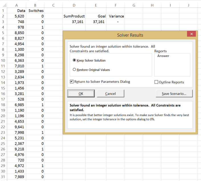
If there are no possible solutions, the Solver dialogue box will tell you.

One limitation of using this method is that Solver will only pick up the first possible solution. Meaning, if there are multiple solutions this method will only pick up one of them. So use Solver with a measure of caution.
