Time for a bit of a change of pace. Solver is by far the coolest thing I have learned on Excel in recent memory. I still don’t really understand how it works, but the instructions here will allow you to identify certain numbers in a list of numbers that add to a desired result.
Say you have a big list of data (e.g. bank transactions) that looks something like this:
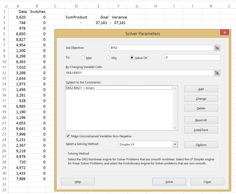
In this example, we have 30 lines of data. A certain combination of these results in 37,161. We want to know which ones will do that.
Switches
This Solver method works on ‘switching’ the appropriate zeros to ones. This will make more sense later but for now, just throw some zeros against each line of data.
SumProduct
If you aren’t familiar with SumProduct don’t worry about it too much. I’ve never used it before this. You can learn more about the function on your own, but for cell D3 the formula is =SUMPRODUCT(A2:A31,B2:B31).
Goal
Simply the number you are aiming for. Manual input.
Variance
Just the difference between the SumProduct cell and the Goal cell.
SOLVER
First thing you’ll need to do is enable the Solver add-in (File > Options > Add-Ins > Pick “Excel Add-ins” from the drop-down menu > Go > Select the “Solver Add-in” checkbox > OK) then open it up in the Data tab.
Without over-explaining things (because I don’t understand how this works and think it’s still mostly magic) this is what your dialogue box should look like:
Don’t ask me why. I don’t know.
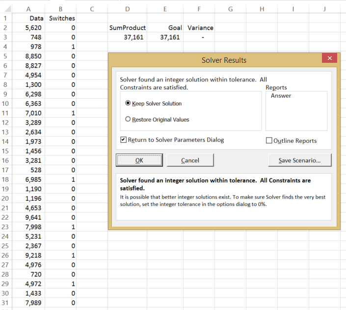
Then hit Solve. The magic Solver pixies will flick the switches of the numbers that add to your specified goal.
Solver will flick the switches from 0 to 1 of the right cells
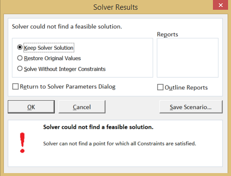
If there are no possible solutions, the Solver dialogue box will tell you.
Solver pixies hate you
One limitation of using this method is that Solver will only pick up the first possible solution. Meaning, if there are multiple solutions this method will only pick up one of them. So use Solver with a measure of caution.
Alternative title: that-one-time-my-colleagues-convinced-me-to-throw-my-money-in-the bin.xlsx
Bit of backstory, not like you need it. My colleagues somehow convinced me to buy into their syndicate for the Euromillions. I suspect they wanted me in because I’m the only accountant amongst them and they needed me to track of whether or not we won. Pooling all our money together, we were able to buy 50 lottery tickets and just like that, we were in with a chance to win £155m! Spoiler alert – we didn’t win.
The lottery worked by drawing 5 Main Numbers and 2 Lucky Stars. There were 50 possible Main Numbers and 12 possible Lucky Stars with various structures of MN and LS resulting in various potential winnings. For example, 5MN+2LS was the jackpot of £155m whilst 2MN+0LS was the lowest winning structure, returning a handsome £3.30.
You think I’d be writing this shit if I won £12.4m?
Above shows the syndicate tracker. I won’t go into it much but it just shows how much each person would win based on the different win structures. Nothing too complicated but it was useful because not everybody contributed the same amount to the syndicate.
Excerpt of our win loss tracker
Now for the juicier stuff. There’s quite a few sections in the image above so we’ll take it one section at a time.
Data Entry
Columns A to H is pure data entry. I manually entered the winning numbers for each ticket we bought, each number in a separate cell. Nothing complicated about that. I did put a conditional format in these cells to highlight that green colour based on any matches to the actual drawn numbers (O2 to U2).
Drawn Numbers
Cells O2 to U2 are the actual numbers drawn on the night. Again, just a manual input. I also used these cells prior to the draw to play out a few random scenarios to get a feel of what the expected payout was going to be.
Ticket Number Frequencies
Columns O to T, rows 13 to 35 has some basic analysis of the numbers in our 50 tickets. It just counts how many instances of each number come up in our tickets. Nothing too interesting – just used the =COUNTIF function. I guess it was interesting that we had at least one instance of every possible number.
Win Structure Lookup
Sorry for jumping around everywhere but I’m getting through the simple stuff before moving onto the complicated bits. Columns W and X is the win structure table. “5&2” refers to 5 matching MN’s with 2 matching LS’s, and so on. This was entirely manually input. Columns Y and Z are purely there for informational purposes only. Look at those win probabilities!
Determining Each Ticket’s Win Structure
OK this brings us to columns J to M. Column J counts the number of MN’s in each ticket that match the actual drawn numbers. Similarly, column K counts the number of LS’s in each ticket that match the actual drawn numbers. Column L combines the two in a format that matches the Win Structure lookup table then Column M shows the corresponding winnings that particular win structure pays out.
Results Summary
Finally this brings us to the small box in the middle. This gives a few stats in an easy to read format: 1) Total Return: sum of column M 2) Number of Winning Tickets: number of non-zero results in column M 3) Return per Share: we had 12.5 shares so it was just Total Return/12.5 4) Net Return per Share: each share cost £10, so this was simply the Return per Share, less the cost
Four winning tickets out of 50, with a net loss of £7.92 per share. Not a great result but it was a fun exercise anyway. Playing with some random scenarios prior to the draw was quite fun and it was a good exercise in performing various count functions.
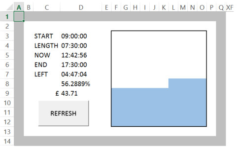
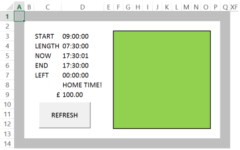
There’s usually not a hell of a lot to do during the day so I need to find ways to occupy my time (hence this blog thing). One of the first things I made in this job was TIME.xlsx which visually tracks how much of my working days is left before I can go home. The idea was to have something resembling an hourglass I could stare at to remind myself that time had not stood still and every second that passed was a second closer to going home or the sweet release of death.
Only 56.2889% of the day left
The best thing about my work day
The big square fills up as the day progresses until the end of the day where the box is full and the squares turn green. Apart from the times, the numbers on the left also show the percentage of the day remaining (D8) and how much I have earned at any point in the day (D9). The big REFRESH button is there because sometimes the sheet does not refresh on its own so I recorded a macro to do it with the click of a button. Yes it’s easier to just hit F9 but it’s more satisfying to click a macro button OK. Though I will admit it is satisfying to hold F9 and watch the numbers fly up tiny increment at a time.
Method
The Numbers
Going from top to bottom we first have the start time in D3, which is the time you clocked in to work. I always start work at the same time so I basically never need to touch this cell. Making sure the cell is set to the ‘Time’ number format, input the time in HH:MM:SS format. I start work at 9am, so that will be 09:00:00.
Next we have the length of your working day. I have a 7.5hr standard work day so again with the same format, I put in 07:30:00. I do have a 1hr lunch break but we’ll get to that.
The next number down is interesting. I needed to get the current time on the sheet at any one point. To do so, I used the =NOW function. The problem with this function is that it also gives the day, not just the time. Without getting too much into it*, this messes up all the other formulas so to remove the day component of the function the full function is “=NOW()-TODAY()”.
The number below is the time I am expecting to finish work. This is basically the start time, add the length of my work day and add my lunch break. My lunch break is an hour, so the formula needs to add TIME(1,0,0) to everything else.
The next number is the amount of time left in my day, again in the HH:MM:SS format. This is simply the time I am expecting to finish work, subtract the current time. To stop this number from going negative after my working day is finished I used an IF function to show a nil value if the aforementioned formula results in a negative number.
The percentage of the working day remaining comes next. This is simply the remaining time (see above) divided by the total time. Because I’m cute af, I made it say “HOME TIME!” when the percentage reaches zero.
And finally because I’m a money ho, I have the amount of money I have earned at any given time on the sheet too. This is simply my daily earnings multiplied by the portion of the day that has passed (1 less the percentage of the working day remaining). This errors when the working day is finished, so I used the IFERROR function to show my full day rate, instead of the formula, when the day is over.
The Box
There is almost definitely a smarter way of doing this, but I’m dumb and lazy so this is how I did it. The box itself is a 10×10 grid. To make it a square I just made the column widths the same number of pixels as the column height. Outside of the visible area (I used columns R to AA) I filled a separate 10×10 area with percentages from 1% to 100%. This is where the box will look up. The formula within the box has 3 possible outcomes – 0, 1 or 2. Using an IF formula I made the following statements: if the amount of time left in the day (D8) is greater than the cell’s equivalent lookup cell then show “0”. If the cell showing the amount of time left in the day shows “HOME TIME!” (that is, when there is 0% of the day left) show “2”. In all other instances show “1”. Then quite simply I put three conditional formats into that area. Have white font and a white background for cells with a “0” result. Have blue font and a blue background for cells with a “1” result. And have green font and a green background for cells with a “2” result. That way, we just have coloured cells without the numbers visible.
And that’s it really. Not too complicated but it has a few lessons on using time functions and somewhat creative formatting methods.
This is a space for me to waste time at work while keeping track of various Excel-based tools I have created while wasting time at work. Some people doodle with a pen and paper, I do my doodling with a spreadsheet and formulas.
This place will be pretty casual. Sometimes there will be tips, sometimes tricks, sometimes tools I have made. The only consistent thing will be that it will all be poorly written. Feel free to ask questions or critique anything. I actually enjoy learning more about Excel and hey, it will help me pass time at work.